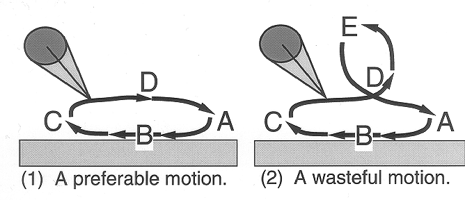
(Figure 2: Crawling motions of the robot arm.)
In order to explain the features of practical RL tasks, we take up a robotics example. Consider a planar two-link manipulator in a gravitational environment as shown in Figure 1. The robot has to move to the front, but the agent does not have any knowledge about the environment previously. At each time step, the agent observes noisy sensor-readings of the joint angles, and outputs turning direction of the joint motors. The immediate reward is defined as the distance of the body movement by the step. In order to move the body to the front, the arm should be controlled as if it is crawling. Through trial and error, the agent has to learn such a control policy that maximizes reward function. The environment is considered to be a partially observable Markov decision processes (POMDPs) which has continuous state space.
This kind of tasks have the following 3 difficulties.
(1) Delayed Reinforcement:
The agent should learn the movement as the right-hand side of Figure 2.
When the arm is touching the ground and moving as A-B-C,
then positive immediate reward is given,
so the agent can learn this movement easily.
On the other hand, the movement C-D-A gives zero immediate reward.
If the arm is moving wastefully like
C-D-E-D-A shown in the left-hand side of Figure 2,
then the agent is given the same zero immediate reward.
Accordingly, the agent has to learn appropriate actions
by delayed reinforcement.

(Figure 2: Crawling motions of the robot arm.)
(2) Hidden state problems arise from imperfect state observation owing to noisy or insufficient sensors. We think that POMDPs represent the hidden state problem.
(3) Function approximation:
In order to generalize large and continuous state space,
the agent has to use function approximators.
There are many ways to do it;
neural networks, fuzzy logic systems, etc.
The simplest way is quantizing:
partitioning the continuous state space into
multidimensional grid, and treating each cell as an atomic object.
The grid approach has a number of dangers.
Increasing the resolution costs computational resource
and physical amount of data exponentially
(Moore, A.W and Atkeson, C.G.: The Parti-game Algorithm for
Variable Resolution Reinforcement Learning in Multidimensional
State-spaces, Machine Learning, 21, pp.199-233, 1995).
In addition, the cells which are roughly partitioned have hidden state.
This robot has the same POMDP problem.
Assume that the continuous sensor-readings are partitioned into
4 discrete cells as shown in Figure 3.
Then the observation X1 includes two hidden states:
one is that the arm top is touching the ground, the other is not.
The difficulties of this example can be theoretically generalized to a decision problem in POMDPs using function approximators.
The objective of the agent is to form a stochastic policy, that assigns a probability distribution over actions to each observation, so that maximize some reward function. The policy is represented by a parametric function approximator using the internal variable vector W. The agent can improve the policy function by means of modifying W.
We have presented a RL algorithm in POMDPs, that is based on a stochastic gradient ascent on discounted reward. It uses function approximator to represent a stochastic policy, and updates the policy parameters. We believe it is the most hopeful approach in that case.
See the detail of the algorithm.